

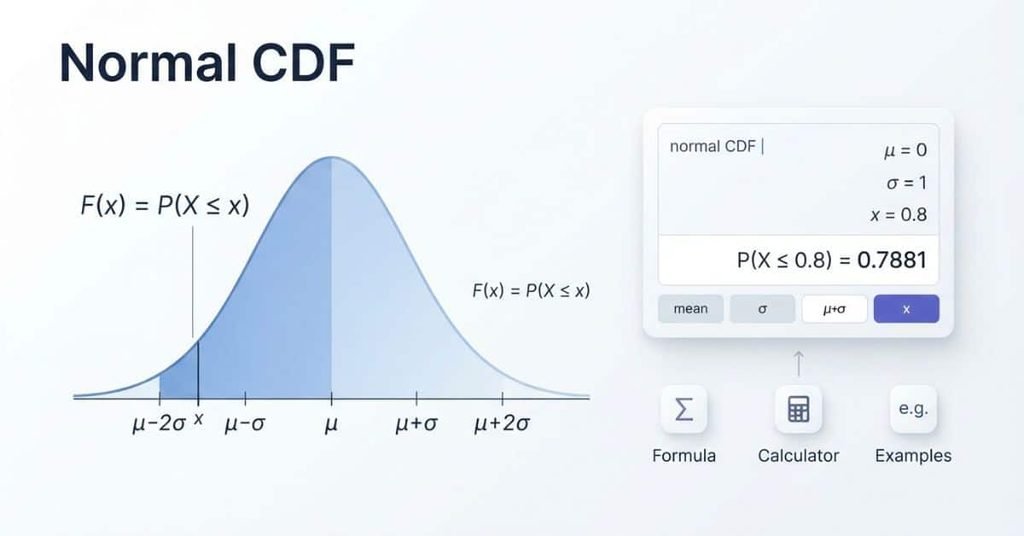
Table of Contents
Introduction
Ever wondered how statistics turns a single score into a probability?
If you need to know the chance of a normal variable falling below a value, the normal CDF is the tool you need. Learning how to calculate normal CDF helps you solve probability questions in statistics, exams, and real-world data analysis.
For beginners, the notation can look confusing at first. The good news is that the process becomes simple once you understand z-scores and cumulative probability.
In this guide, you will learn how the normal CDF works and how to calculate it step by step. You will also see how to use a normal CDF calculator, calculate normal CDF by hand, and find it on a TI-84.
By the end, you will know which method to use and how to interpret your answer confidently.
What Is the Normal CDF?
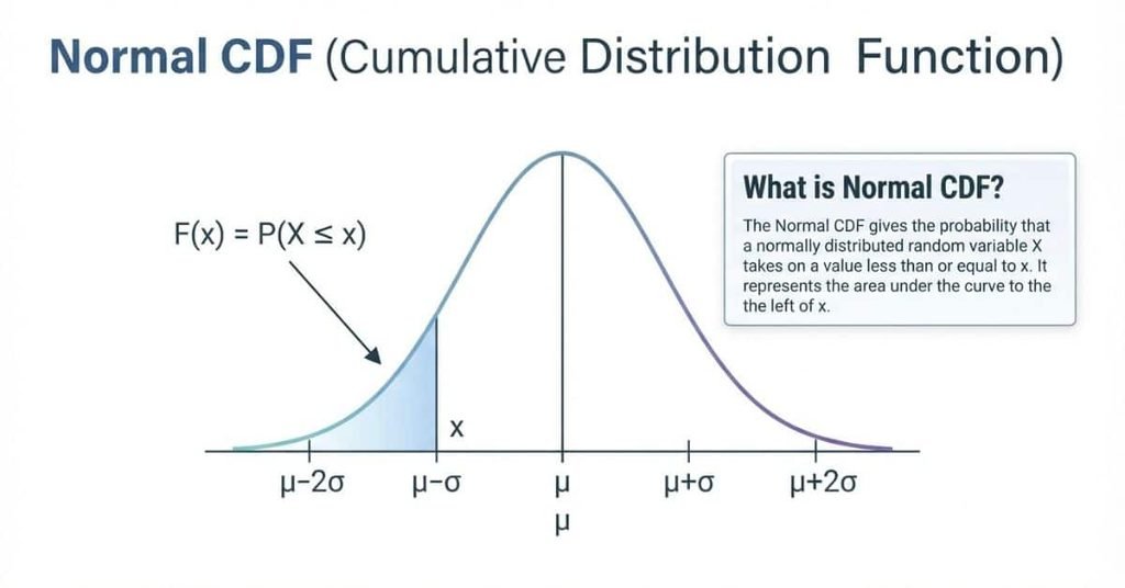
The normal cumulative distribution function (CDF) gives the probability that a normally distributed variable is less than or equal to a specific value. It measures the area under the normal curve up to that point.
The normal CDF is written as:
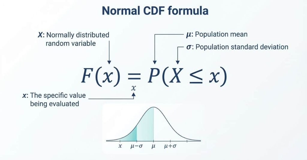
Here’s what each symbol means:
- XX — the normally distributed random variable.
- xx — the specific value you want to evaluate.
- PP — the probability of an event occurring.
- F(x)F(x) — the cumulative probability up to .
For example, suppose test scores follow a normal distribution. You might want to find the probability that a randomly selected score is 70 or lower. The normal CDF can give you that probability.
The result is always between 0 and 1. You can also express it as a percentage. For example, a CDF value of 0.80 means an 80% probability of observing a value at or below .
Need a faster way to calculate cumulative probability? Use our Normal CDF Calculator to get accurate results without doing the calculations manually.
What Does CDF Tell You?
Suppose you want to find:
The CDF tells you the area under the normal curve to the left of 70. That area represents the probability that is 70 or less.
Think of the normal curve as a smooth hill. The CDF simply adds up all the probability from the far left of the curve through your chosen value.
This idea is the foundation for using a normal CDF calculator, a statistical table, or a calculator such as the TI-84.
Normal CDF Formula
The normal CDF uses a simple probability function to describe values up to a chosen point:
For a normal distribution, we write:
Here, μ\mu represents the mean, while σ\sigma represents the standard deviation. The mean shows the center of the distribution. The standard deviation describes how spread out the values are.
When you calculate a normal CDF, you are finding the probability that falls at or below a specific value . The result represents the area under the normal curve to the left of that value.
Although calculus can describe the normal CDF through an integral, beginners usually don’t need to evaluate that integral manually. A normal CDF calculator, statistical software, or calculator such as the TI-84 can evaluate the probability quickly.
This makes the formula easier to use in practical probability problems. You mainly need the value, mean, and standard deviation to get started.
How to Calculate Normal CDF
Calculating a normal CDF becomes straightforward when you follow the same four steps each time. You need the distribution’s mean, standard deviation, and the X value you want to evaluate.
Step 1 — Identify the Mean and Standard Deviation
Start by identifying the mean and standard deviation of your normal distribution. For this example, assume:
The mean, , represents the center of the distribution. The standard deviation, , shows how far values typically spread from that center.
Step 2 — Identify the X Value
Next, identify the value for which you want the cumulative probability. Suppose the value is:
Your goal is to find the probability that a randomly selected value is 85 or lower.
Step 3 — Convert X to a Z-Score
Convert the X value into a standard score using:
Substitute the values:
So, 85 is 1.5 standard deviations above the mean.
Step 4 — Find the Cumulative Probability
Now convert the problem into a standard normal probability:
Use a calculator, statistical software, or standard normal table to find the cumulative probability.
For , the CDF is approximately:
Therefore:
This means there is about a 93.32% probability that is 85 or lower.
After learning the formula, try the Normal CDF Calculator to check your answer and practice with different mean, standard deviation, and X values.
How to Calculate Normal CDF Using a Calculator
A Normal CDF Calculator makes cumulative probability problems faster and easier. Instead of converting values by hand, you can enter the distribution details and get the probability directly.
Depending on the calculator design, you typically enter:
- Lower bound: The starting value for the probability range.
- Upper bound: The ending value for the probability range.
- Mean (μ\mu): The center of the normal distribution.
- Standard deviation (σ\sigma): The spread of the distribution.
For a probability such as , use a suitable lower bound and enter your target value as the upper bound. The calculator then evaluates the area under the normal curve between those values.
Example Using a Normal CDF Calculator
Suppose test scores have a mean of 75 and a standard deviation of 8. Find the probability that a randomly selected score is 85 or lower.
Start with:
Enter the following values:
- Lower bound:
- Upper bound:
- Mean:
- Standard deviation:
The corresponding z-score is:
The cumulative probability is approximately:
So, the probability is approximately 89.44%.
Try the Normal CDF Calculator to check your answer and practice with different values.
How to Calculate Normal CDF by Hand
You can calculate a normal CDF by hand using a Z-score and a standard normal table. This method helps you understand what a normal CDF calculator does behind the scenes.
The process has three main steps. First, convert your value into a Z-score. Next, find that Z-score in a standard normal table. Finally, read the cumulative probability from the table.
Step 1 — Calculate the Z-Score
Start by converting the raw value into a standard score. Use this formula:
Z-score formula:
z = (x − μ) ÷ σ
Here, x is your value, μ is the mean, and σ is the standard deviation.
Using the earlier example:
- x = 85
- μ = 75
- σ = 8
Substitute these values:
z = (85 − 75) ÷ 8
z = 10 ÷ 8 = 1.25
So, the Z-score is 1.25.
Step 2 — Use a Standard Normal Table
Next, find 1.25 in a standard normal Z-table. Most Z-tables organize values using the first two digits and the hundredths place.
For (z=1.25), locate:
- Row: 1.2
- Column: 0.05
- Table value: 0.8944
Different tables may use slightly different formats. Always check the table’s heading and instructions before reading a value.
Step 3 — Read the Cumulative Probability
The table value represents the cumulative probability to the left of the Z-score.
For (z=1.25):
P(Z ≤ 1.25) = 0.8944
This means about 89.44% of values fall at or below this Z-score.
The Z-score itself is not the probability. The Z-score tells you the position relative to the mean. The table converts that position into cumulative probability.
Example
Suppose test scores have a mean of 75 and a standard deviation of 8. Find the probability that a randomly selected score is 85 or lower.
Start with:
P(X ≤ 85)
Calculate the Z-score:
z = (85 − 75) ÷ 8 = 1.25
Then use a standard normal table:
P(Z ≤ 1.25) = 0.8944
Therefore:
P(X ≤ 85) = 0.8944
So, the probability is approximately 89.44%.
This gives the same result as the normal CDF calculator method. The difference is that you found the probability manually instead of using technology.
How to Calculate Normal CDF Without a Calculator
If you do not have a calculator, you can still calculate a normal CDF. The most common option is a standard normal Z-table.
A printed statistical table works in the same basic way. First, calculate the Z-score. Then, find that value in the table and read its cumulative probability.
Standard Normal Z-Table
A Z-table is the easiest manual method for most students. It provides cumulative probabilities for standard normal Z-scores.
For example, if your calculation gives:
z = 1.25
The standard normal table gives:
P(Z ≤ 1.25) = 0.8944
So, the normal CDF is 0.8944, or 89.44%.
Printed Statistical Tables
Printed statistics books often include normal distribution tables. These tables may display cumulative probabilities, areas between values, or areas in a different format.
Always check what your specific table represents. Not every Z-table uses the same layout.
If you want to calculate normal probabilities quickly, our Normal CDF Calculator lets you enter your values and find the cumulative probability in seconds.
Approximation Methods
You can also estimate normal CDF values using numerical approximation methods. However, these methods are usually unnecessary for basic statistics problems.
For most students, a Z-table provides the simplest manual solution.
Remember that the Z-score is not the CDF. A Z-score such as 1.25 only tells you how far a value lies from the mean. You still need a Z-table, statistical table, software, calculator, or numerical approximation to obtain the CDF.
For exact practical calculations, technology is usually faster. For learning and exams, knowing how to use a Z-table remains useful.
How to Calculate Normal CDF on a TI-84
The TI-84 can calculate a normal CDF quickly using its built-in normalcdf function. This is useful when you need accurate cumulative probabilities without using a Z-table.
TI-84 Normal CDF Steps
On most TI-84 calculators, open the normal CDF function with:
2nd → VARS → normalcdf(
The calculator uses four main arguments:
normalcdf(lower, upper, μ, σ)
These values represent:
- Lower: Starting value of the range
- Upper: Ending value of the range
- μ: Mean
- σ: Standard deviation
Suppose you want to calculate:
P(X ≤ 85)
Use the earlier example:
Use the earlier example:
- Lower: A very small value
- Upper: 85
- Mean: 75
- Standard deviation: 8
For the lower bound, you can use a sufficiently small number, such as -1E99. This represents a value far into the left tail.
Enter:
normalcdf(-1E99, 85, 75, 8)
The TI-84 returns approximately:
0.8944
So:
P(X ≤ 85) ≈ 0.8944
The probability is therefore 89.44%.
Why Use Such a Low Lower Bound?
A normal distribution technically extends toward negative infinity. For a left-tail probability, you want to include virtually the entire distribution below 85. A very small lower bound effectively represents −∞ for the calculator.
Always enter the values in the correct order. Switching the mean or standard deviation can produce an incorrect result.
How to Calculate Normal CDF for Different Probability Regions
Normal CDF problems can ask about different parts of a normal distribution. The method depends on whether you need the area below, above, between, or outside specific values.
The key idea is to use the CDF, (F(x)), to find cumulative probability. You can then subtract or complement CDF values when the problem covers another region.
Probability Below X
A probability below a value represents the left-tail probability:
P(X ≤ x)
This is the normal CDF itself:
P(X ≤ x) = F(x)
For example:
P(X ≤ 85) = 0.8944
The result tells you the proportion of observations at or below 85.
Probability Above X
A probability above a value represents the right-tail probability:
P(X ≥ x)
Use the complement of the CDF:
P(X ≥ x) = 1 − P(X ≤ x)
For the earlier example:
P(X ≥ 85) = 1 − 0.8944
P(X ≥ 85) = 0.1056
So, approximately 10.56% of values are 85 or higher.
Probability Between Two Values
To find the probability between two values, subtract the lower CDF from the upper CDF:
P(a ≤ X ≤ b) = F(b) − F(a)
For example, suppose you want:
P(70 ≤ X ≤ 85)
With a mean of 75 and standard deviation of 8:
F(85) = 0.8944
For 70:
z = (70 − 75) ÷ 8 = −0.625
The corresponding cumulative probability is approximately:
F(70) ≈ 0.2660
Therefore:
P(70 ≤ X ≤ 85) = 0.8944 − 0.2660
P(70 ≤ X ≤ 85) ≈ 0.6284
So, the probability is approximately 62.84%.
Probability Outside Two Values
An outside probability includes both tails of the distribution. For example:
P(X ≤ a or X ≥ b)
You can calculate each tail separately:
P(X ≤ a) + P(X ≥ b)
For the right tail, use the complement:
P(X ≥ b) = 1 − F(b)
Therefore:
F(a) + [1 − F(b)]
This approach helps you avoid confusing the middle region with the two outside tails. When using a normal CDF calculator, calculate each tail and add the two probabilities.
Normal CDF Example With Two Bounds
A normal CDF can also find the probability that a value falls between two numbers. In this case, subtract the lower cumulative probability from the upper cumulative probability.
Suppose exam scores are normally distributed with a mean of 72 and a standard deviation of 10. What is the probability that a student scores between 65 and 80?
Set up the probability:
P(65 ≤ X ≤ 80)
Step 1: Find the Z-Score for 80
Use the Z-score formula:
z = (x − μ) ÷ σ
For x = 80:
z = (80 − 72) ÷ 10 = 0.8
The standard normal CDF for z = 0.80 is approximately:
F(80) = 0.7881
Step 2: Find the Z-Score for 65
For x = 65:
z = (65 − 72) ÷ 10 = −0.7
The standard normal CDF for z = −0.70 is approximately:
F(65) = 0.2420
Step 3: Subtract the Two CDF Values
Use the formula:
P(65 ≤ X ≤ 80) = F(80) − F(65)
Substitute the values:
P(65 ≤ X ≤ 80) = 0.7881 − 0.2420
P(65 ≤ X ≤ 80) = 0.5461
Therefore, the probability is approximately 54.61%.
The same result can be found with a normal CDF calculator. Enter 65 as the lower bound, 80 as the upper bound, 72 as the mean, and 10 as the standard deviation.
What Is an Inverse Normal CDF?
A normal CDF starts with a value and finds its cumulative probability. An inverse normal CDF works in the opposite direction.
With a normal CDF, you ask:
Given (X), what is the probability?
With an inverse normal calculation, you ask:
Given the probability, what value of (X) produces it?
For example:
P(X ≤ x) = 0.95
Here, the probability is already known. Your goal is to find the value x that marks the 95th percentile.
For a standard normal distribution, the 95th percentile has a Z-score of approximately:
z = 1.645
If the distribution has a mean of 75 and a standard deviation of 8, convert that Z-score back to the original scale:
x = μ + zσ
x = 75 + (1.645)(8)
x ≈ 88.16
So, approximately 88.16 represents the 95th percentile for this distribution.
An inverse normal calculator makes this process much faster. If your calculator includes an Inverse Normal Calculator, you can enter the desired cumulative probability, mean, and standard deviation to find the corresponding cutoff value.
Normal CDF vs. Inverse Normal
| Normal CDF | Inverse Normal |
|---|---|
| X → Probability | Probability → X |
| Finds cumulative area | Finds a cutoff value |
| Example: (P(X\le85)) | Example: 95th percentile |
| Starts with a value | Starts with a probability |
The key difference is the direction of the calculation. Normal CDF finds area, while inverse normal finds the value associated with that area.
Common Normal CDF Mistakes
Normal CDF problems become much easier when you know which values and probability regions you need. These common mistakes can lead to incorrect answers even when the calculation looks simple.
Confusing CDF With PDF
The PDF and CDF describe different things.
- PDF: Describes probability density at different values.
- CDF: Gives cumulative probability up to a specific value.
For a normal distribution, the CDF answers:
P(X ≤ x)
A PDF value should not be interpreted directly as the probability below x.
Using the Wrong Standard Deviation
When calculating a normal CDF, σ must be the standard deviation.
Do not enter the variance in its place. Variance equals the standard deviation squared:
σ² = variance
If you only have the variance, take its square root first:
σ = √variance
Using variance instead of standard deviation can change the final probability significantly.
Forgetting to Standardize
When using a standard normal table, you usually need to convert x into a Z-score first.
Use:
z = (x − μ) ÷ σ
You do not need this manual step when a calculator accepts the raw value, mean, and standard deviation directly.
Using the Wrong Tail
Pay close attention to whether the problem asks for values below or above x.
For values below x:
P(X ≤ x) = F(x)
For values above x:
P(X ≥ x) = 1 − F(x)
Choosing the wrong tail can turn a small probability into a large one.
Confusing CDF With Inverse CDF
A normal CDF starts with an X value and finds its probability.
An inverse CDF starts with a probability and finds the corresponding X value.
For example:
P(X ≤ 85)
uses a known value to find probability. In contrast:
P(X ≤ x) = 0.95
uses a known probability to find the cutoff value x.
Remember the direction before choosing a calculator function.
Normal CDF vs. Z-Score
A Z-score and a normal CDF are closely related, but they do different jobs. Understanding this difference helps prevent one of the most common beginner mistakes.
A Z-score tells you how many standard deviations a value is from the mean. It standardizes a raw value so you can compare its position within a distribution.
The formula is:
z = (x − μ) ÷ σ
For example:
z = 1.5
This means the value is 1.5 standard deviations above the mean.
However, 1.5 is not the probability. To find the cumulative probability, you use the normal CDF:
P(Z ≤ 1.5)
The standard normal CDF gives approximately:
P(Z ≤ 1.5) = 0.9332
So, the Z-score describes position, while the CDF describes cumulative probability.
| Z-Score | Normal CDF |
|---|---|
| Measures distance from the mean | Measures cumulative probability |
| Expressed in standard deviations | Expressed as probability or percentage |
| Example: z = 1.5 | Example: P(Z ≤ 1.5) = 0.9332 |
| Used to standardize a value | Converts position into cumulative probability |
The easiest way to remember the difference is: Z-score tells you where you are; CDF tells you how much probability lies below you.
When Should You Use a Normal CDF?
Use a normal CDF when you need the probability that a normally distributed value falls below, above, or between specific values.
Common student examples include:
- Exam scores: Find the percentage of students scoring below a certain score.
- Heights: Calculate the probability that a randomly selected person falls within a height range.
- Test results: Find the chance of getting a score above or below a target.
- Measurement errors: Estimate how often a measurement falls within a specific range.
- Percentiles: Find the cumulative percentage below a particular value.
- Probability questions: Solve problems involving areas under a normal distribution.
- AP Statistics problems: Calculate probabilities for normally distributed variables using a calculator or Z-table.
For example, if exam scores have a known mean and standard deviation, you can use the normal CDF to find:
P(X ≤ 85)
You can also calculate probabilities such as:
P(70 ≤ X ≤ 85)
In short, use a normal CDF whenever a problem asks how much probability lies below, above, or between values in a normal distribution.
Conclusion
Understanding how to calculate normal CDF makes many probability problems easier to solve. This guide covered formulas, Z-scores, Z-tables, calculators, and TI-84 methods.
You also learned how to calculate probabilities below, above, between, and outside selected values. The examples showed how each method produces the same probability when used correctly.
Remember that a Z-score shows position, while a CDF gives cumulative probability. An inverse normal calculation works in the opposite direction.
With regular practice, normal CDF problems become much more manageable. Try different values to build confidence with each method.
Explore more statistics resources on our website for additional practice. You can also share this guide with classmates who are learning normal distributions.
The normal CDF gives the cumulative probability that a normally distributed variable is less than or equal to a specific value.
Calculate the Z-score using the formula below. Then use a Z-table, calculator, software, or normal CDF function to find the cumulative probability.
First, calculate the Z-score. Next, find the Z-score in a standard normal table. The table value gives the cumulative probability P(Z ≤ z).
Use a standard normal Z-table or printed statistical table. Calculate the Z-score first, then find its cumulative probability in the table.
Press 2nd → VARS → normalcdf(. Enter the lower bound, upper bound, mean, and standard deviation.
For a left-tail probability, use a very low lower bound to represent the far-left tail of the normal distribution.
The basic normal CDF formula is:
For a normal variable, X follows a normal distribution with mean μ and standard deviation σ.
A PDF describes probability density across possible values. A CDF gives cumulative probability up to a specific value.
The CDF represents the accumulated area under the PDF.
Inverse normal CDF finds an X value from a given cumulative probability. For example, it can find the score representing the 95th percentile.
Subtract the lower cumulative probability from the higher cumulative probability.
This gives the probability between the two Z-scores.

Team ClassRank builds smart, student-friendly calculators to make grade and rank tracking simple and accurate. For questions or feedback, contact us at classrankcalculator@gmail.com.