Density Curve in Statistics: Definition, Examples & Height

Introduction

What if you could understand a probability distribution just by looking at its shape?

A density curve gives you a simple way to understand how numerical data is distributed. It is especially useful in statistics because it connects the shape of data with probability and area. For beginners, the idea can seem confusing at first. The good news is that the basic rules are easier than they look.

In AP Statistics and introductory college courses, density curves appear in many probability problems. You may need to find the height of a curve, interpret the area under it, or understand a normal distribution.

In this guide, you will learn what a density curve is and how it works. You will also see clear density curve examples with simple calculations. We will explain uniform and normal density curves step by step.

By the end, you will know how to interpret density curves and solve common statistics problems with confidence.

What Is a Density Curve?

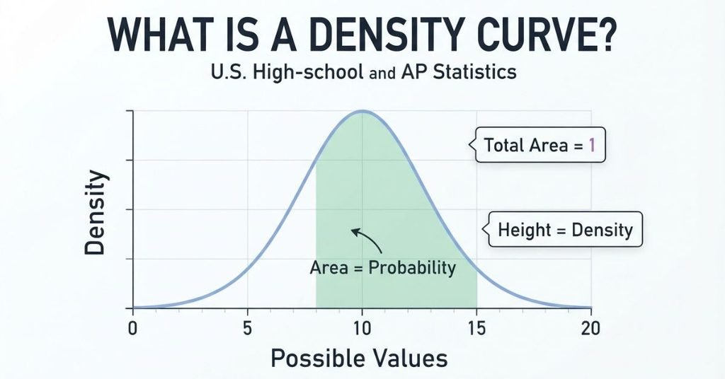
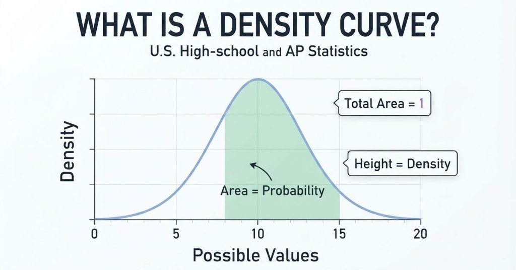
A density curve is a smooth graph that describes how values are distributed for a continuous random variable. It shows where values tend to occur and helps you understand probability using area.

Need to check your calculations? Use our Density Curve Calculator to find density, height, area, and probability quickly

A density curve has possible values on the x-axis. The curve’s height shows the relative density of values at each point. A taller curve means values are more concentrated around that location.

The total area under a density curve always equals 1. This represents the total probability of all possible outcomes. The area between two x-values represents the probability that a value falls within that range.

Because density curves model continuous distributions, individual points have zero probability. Instead, probability comes from intervals and their areas. Common examples include uniform and normal density curves.

What Are Density Curves Used For?

Density curves help statisticians describe distributions and calculate probabilities for continuous variables. They provide a visual way to connect data values with probability.

Students commonly use density curves to:

• Find probability: Use the area under the curve to find probabilities.
• Describe distributions: Understand the shape and spread of a continuous distribution.
• Study continuous variables: Model measurements such as height, weight, time, or temperature.
• Support statistical inference: Use probability models when estimating or testing claims about populations.

Expert Tip: Always remember the key idea: height describes density, while area represents probability. This distinction prevents many common mistakes in AP Statistics.

Properties of a Density Curve

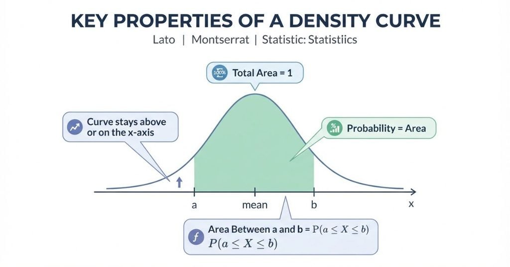
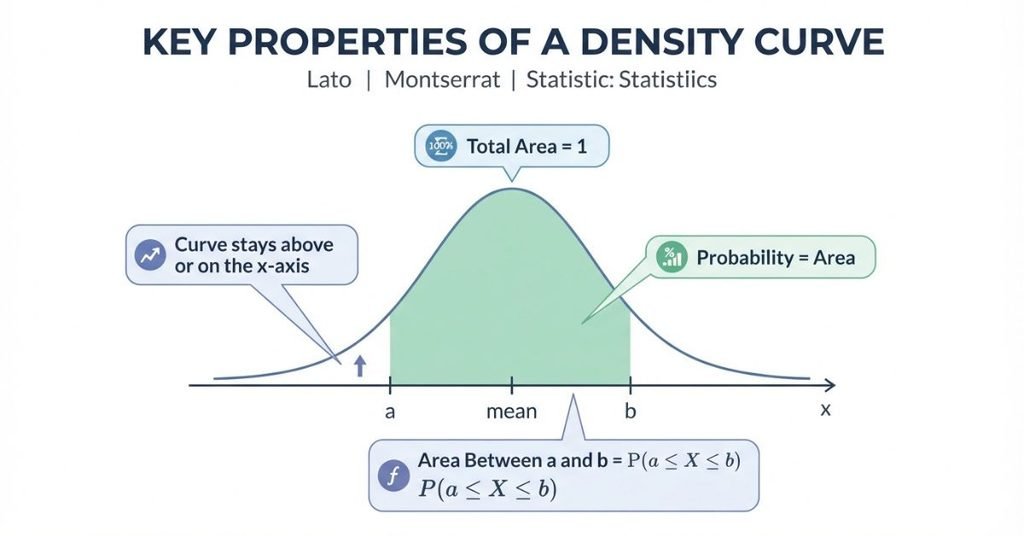
A density curve follows a few important rules. Learning these rules makes probability questions much easier.

1. The curve cannot go below the x-axis. Density cannot be negative, so every part of the curve stays at or above zero.
2. The total area under the curve equals 1. The entire area represents all possible outcomes. Therefore, total area equals 1, or 100% probability.
3. Probability is represented by area. The height of a curve shows density at a particular value. Height alone does not give the probability of an outcome.
4. Area between two values represents probability. For values from $a$ to $b$, the probability is written as $P(a \le X \le b)$. You find this probability by measuring the area under the curve between $a$ and $b$.

A Density Curve Cannot Be Below the X-Axis

Density values cannot be negative. A negative height would create negative area, which cannot represent probability. For this reason, every valid density curve stays on or above the x-axis.

Total Area Under the Curve Equals 1

The entire area under a density curve represents every possible value of the variable. Since all possible outcomes have a total probability of 100%, the complete area must equal 1.

Probability Is Represented by Area

Height and probability are not the same thing. A curve can have a high point, but that height alone does not tell you the probability.

For continuous variables, probability comes from an interval of values. The wider the interval, the more area it may contain.

Area Between Two Values Represents Probability

Suppose you want the probability that $X$ falls between $a$ and $b$. You write it as:$$P(a \le X \le b)$$

This probability equals the area under the density curve from $a$ to $b$.

You can also use the Density Curve Calculator to explore how changes in the interval affect the curve’s height and area.

How Does a Density Curve Work?

Think of a density curve as a map of where values are concentrated. The height shows density, while the area shows probability.

For example, imagine a uniform density curve from 0 to 10. The curve has the same height across the entire interval. If you want the probability that $X$ falls between 2 and 6, you find the area from 2 to 6.

That interval covers 4 out of 10 equal units. Therefore:$$P(2 \le X \le 6)=\frac{4}{10}=0.40$$

So the probability is 0.40, or 40%. The complete area from 0 to 10 equals 1.

Expert Tip: When solving density curve problems, ask one question first: “Am I looking for height or area?” Height describes density. Area gives probability.

How to Find the Height of a Density Curve

Finding the height of a density curve depends on the type of curve you are studying. For a uniform density curve, the height stays constant across its entire range.

You can find this height by using the total area under the curve. Since the total area must equal 1, the curve’s base and height must multiply to 1.

This makes uniform density curves especially easy to solve. You only need the lower and upper bounds of the distribution.

Height vs. Probability

Height and probability describe different ideas. Height represents density, while area represents probability.

A higher curve does not automatically mean a higher probability. You must consider both the height and the width of the interval.

For a continuous variable, the probability at one exact point is zero. Probability comes from the area across an interval.

Finding Height From Area

For a uniform density curve, the graph forms a rectangle. You can use the familiar rectangle formula:$$\text{Area}=\text{Base}\times\text{Height}$$

Because the entire density curve has an area of 1:$$1=\text{Base}\times\text{Height}$$

You can then divide 1 by the base to find the height.

---

How to Find the Height of a Uniform Density Curve

A uniform density curve has the same height across its entire range. If the lower bound is $L$ and the upper bound is $U$, the base equals $U-L$.

Use this formula:$$\boxed{\text{Height}=\frac{1}{\text{Upper Bound}-\text{Lower Bound}}}$$

This formula works because the complete area under every density curve must equal 1.

Step-by-Step Example

Suppose a uniform density curve ranges from 2 to 8.

Step 1: Find the base.$$8-2=6$$

Step 2: Apply the height formula.$$\text{Height}=\frac{1}{6}$$

Step 3: Convert to a decimal if needed.$$\text{Height}\approx0.167$$

So, the height of the uniform density curve is approximately 0.167.

For a quick way to apply these formulas, try the Density Curve Calculator and compare your results with the calculations.

Why Does the Formula Work?

A uniform density curve forms a rectangle. Its base is the distance between the lower and upper bounds.

The total area must equal 1:$$\text{Base}\times\text{Height}=1$$

Substituting the base $U-L$ gives:$$(U-L)\times\text{Height}=1$$

Dividing both sides by $U-L$ produces the height formula. This ensures the entire curve represents 100% probability.

Expert Tip: Always find the base first. Subtract the lower bound from the upper bound before calculating the height.

What Is a Uniform Density Curve?

A uniform density curve represents a continuous variable with equal density across a specific interval. Its graph has a simple rectangular shape.

The curve has a constant height from the lower boundary to the upper boundary. Every value within that interval has the same density.

The lower boundary marks where the distribution begins. The upper boundary marks where it ends. Values outside this interval have zero density.

The entire rectangle has an area of 1. This represents 100% of the probability. Because the height stays constant, you can find it using the width of the interval.

Uniform Density Curve Example

Suppose $X$ follows a uniform distribution from 0 to 10. The curve extends from 0 to 10 with the same height everywhere.

The base is:$$10-0=10$$

The height is:$$\frac{1}{10}=0.10$$

So the density curve forms a rectangle with a base of 10 and a height of 0.10.

Visual idea: Show a rectangular density curve from 0 to 10, with the constant height labeled 0.10 and the full area labeled 1.

Caption: A uniform density curve has constant height across its entire interval.

Alt text: Uniform density curve from 0 to 10 with constant height and total area of 1.

Finding Probability From a Uniform Density Curve

For a uniform density curve, probability equals the area of the relevant rectangle. Use:$$\text{Area}=\text{Base}\times\text{Height}$$

Suppose you want $P(2\le X\le6)$. The interval has a width of 4, and the height is 0.10.$$P(2\le X\le6)=4(0.10)=0.40$$

Therefore, the probability is 0.40, or 40%.Mean of a Density Curve

The mean of a density curve represents its balance point. Think of the curve as a thin, balanced shape resting on a fulcrum.

The mean gives the distribution’s center based on the values and their density. It does not simply identify the most common value.

For a symmetric distribution, the mean and median occur at the center. This includes symmetric uniform distributions and normal distributions.

For example, a uniform distribution from 0 to 10 has a mean of:$$\mu=\frac{0+10}{2}=5$$

A normal distribution also has its mean at the center of its symmetric bell-shaped curve. If $\mu=70$, the balance point is 70.

Mean vs. Median on a Density Curve

The mean and median both describe the center, but they use different ideas.

Measure	Meaning
Mean	The balance point of the distribution
Median	The value that divides the total area into two equal halves

For a symmetric density curve, the mean and median are equal. In a skewed distribution, they can occur at different locations.

---

How to Find Area Under a Density Curve

The area under a density curve represents probability. The complete area always equals 1, representing 100% probability.

To find the probability between two values, focus on the area under the curve between those x-values:$$P(a\le X\le b)$$

The location of the shaded area tells you what probability you are finding.

• Between two values: Find the area from $a$ to $b$.
• Left tail: Find the area to the left of a chosen value.
• Right tail: Find the area to the right of a chosen value.
• Entire curve: The total area equals 1.

Area Under a Uniform Curve

A uniform density curve forms a rectangle. You can find its area with:$$\text{Area}=\text{Base}\times\text{Height}$$

For example, if a uniform curve ranges from 0 to 10, its height is 0.10. The probability from 2 to 6 is:$$(6-2)(0.10)=0.40$$

So, $P(2\le X\le6)=0.40$, or 40%.

Area Under a Normal Curve

A normal density curve has a smooth bell shape. Its probability comes from the area beneath the curve.

For example, the area to the left of a value represents the probability of getting a value below that point. The area to the right represents the probability of getting a value above it.

Normal probability calculations often use z-scores and standard normal tables or calculators. The key idea stays the same: probability is always represented by area.

Expert Tip: When reading a density curve, look for the boundaries of the shaded region. Those boundaries tell you which probability you need.

What Is a Normal Density Curve?

A normal density curve is a smooth, bell-shaped curve used to model many continuous distributions. It is symmetric around its center.

The center is determined by the mean, written as $\mu$. The curve spreads around this mean based on the standard deviation, written as $\sigma$.

A normal curve extends indefinitely in both directions. Its height gets closer to zero toward the tails but does not reach zero.

Like every valid density curve, the total area under a normal curve equals 1. That entire area represents 100% probability.

Mean and Center

The mean $\mu$ identifies the center of a normal density curve. Because the curve is symmetric, the mean divides the distribution into two equal halves.

Values near $\mu$ appear in the highest part of the curve. Values farther from the mean appear toward the tails.

Changing $\mu$ shifts the entire normal curve left or right. It does not change the curve’s overall bell shape.

Standard Deviation and Spread

The standard deviation $\sigma$ describes how spread out the normal distribution is.

A smaller $\sigma$ produces a narrower, taller curve. A larger $\sigma$ produces a wider, flatter curve.

This makes standard deviation useful when comparing how tightly values cluster around the mean.

Normal Curve Probabilities

Probability under a normal density curve comes from area, not height. To find the probability of an interval, find the area beneath the curve over that interval.

For example, $P(a\le X\le b)$ represents the area between $a$ and $b$. Statistical tools and normal-distribution calculations can help find these areas accurately.

Expert Tip: On a normal curve, identify $\mu$ first. Then use $\sigma$ to understand how far values spread from the center.

Density Curve Examples

The best way to understand density curves is to work through simple examples. Each example shows how the curve connects density, area, probability, and the mean.

Example 1 — Uniform Density Curve

Given: A uniform density curve ranges from 2 to 8.

Formula/Method: Find the width, then use the height formula.$$\text{Height}=\frac{1}{U-L}$$

Calculation:$$\text{Height}=\frac{1}{8-2}=\frac{1}{6}\approx0.167$$

Answer: The uniform density curve has a constant height of approximately 0.167.

Example 2 — Finding Probability From Area

Given: A uniform curve ranges from 0 to 10. Find $P(3\le X\le7)$.

Formula/Method: Use area = base × height.

The height is:$$\frac{1}{10}=0.10$$

Calculation:$$P(3\le X\le7)=(7-3)(0.10)$$$$=4(0.10)=0.40$$

Answer: The probability is 0.40, or 40%.

Example 3 — Finding Height

Given: A uniform density curve ranges from 5 to 15.

Formula/Method: Subtract the lower bound from the upper bound.$$\text{Height}=\frac{1}{U-L}$$

Calculation:$$\text{Height}=\frac{1}{15-5}$$$$=\frac{1}{10}=0.10$$

Answer: The height is 0.10.

Example 4 — Normal Density Curve

Given: A normal distribution has a mean of 70 and a standard deviation of 8.

Formula/Method: Identify the center and spread of the curve.

The mean gives the center:$$\mu=70$$

The standard deviation gives the spread:$$\sigma=8$$

Calculation: The curve centers at 70. Values farther from 70 appear toward the tails.

Answer: The normal curve is centered at 70 with a standard deviation of 8.

Example 5 — Finding Mean

Given: A uniform density curve ranges from 10 to 20.

Formula/Method: For a uniform distribution, average the two boundaries.$$\mu=\frac{L+U}{2}$$

Calculation:$$\mu=\frac{10+20}{2}=15$$

Answer: The mean is 15. It represents the balance point of the distribution.

How to Read a Density Curve

Reading a density curve becomes easier when you know what each part represents. Start with the axes, then examine the curve’s shape and areas.

• X-axis: Shows possible values of the continuous variable.
• Y-axis: Shows density. Its height does not directly equal probability.
• Height: Shows how concentrated the density is around a value.
• Area: Represents probability over an interval.
• Center: Shows the distribution’s central location, often its mean.
• Spread: Shows how widely values extend around the center.
• Symmetry: Shows whether both sides have the same shape.
• Tails: Show the areas far from the center.
• Intervals: Define the range used when finding probability.

For example, a normal curve has a clear center at its mean. Its two sides mirror each other because the distribution is symmetric.

When you see a shaded region, focus on its boundaries. The shaded area represents the probability for that interval or tail.

Expert Tip: Never read probability from curve height alone. First identify the interval, then interpret the area beneath the curve.

If you are practicing density curve problems, the Density Curve Calculator can help you calculate and understand your results step by step.

Density Curve vs. Histogram

A density curve and a histogram can look similar because both show the shape of a distribution. However, they represent different things.

A density curve is a smooth mathematical model of a distribution. A histogram uses bars to display data collected from an actual sample.

Feature	Density Curve	Histogram
Shape	Smooth curve	Bars
Purpose	Models a distribution	Displays observed data
Data type	Continuous model	Observed sample data
Total area	Always equals 1	Does not always equal 1
Height	Represents density	Represents frequency or density
Appearance	Smooth and continuous	Grouped into intervals
Distribution	Theoretical model	Actual data visualization

A histogram groups observations into intervals called bins. The height of each bar shows how much data falls within that interval. The exact height depends on how the histogram is constructed.

A density curve does not show individual observations. Instead, it provides a mathematical model for the overall distribution. Its total area is always 1, representing 100% probability.

Why Do They Look Similar?

A histogram and density curve can have similar shapes when the curve models the distribution shown by the data. For example, a roughly bell-shaped histogram may look similar to a normal density curve.

However, the histogram comes from observed data. The density curve represents an idealized model. The histogram may change when you collect a different sample or choose different bin widths.

Expert Tip: Think of a histogram as the data you observed and a density curve as a model that describes the distribution.

Density Curve vs. Normal Curve

One important idea can prevent a common mistake: every normal curve is a density curve, but not every density curve is normal.

A density curve is a general term for a curve that follows the rules of a probability density. A normal curve is one specific type of density curve with a symmetric, bell-shaped form.

Feature	General Density Curve	Normal Density Curve	Uniform Density Curve
Shape	Can have many shapes	Bell-shaped	Rectangular
Symmetry	May or may not be symmetric	Always symmetric	Symmetric over its interval
Center	Depends on the distribution	Mean μ	Midpoint of the interval
Height	Can vary	Highest near μ	Constant
Tails	Depends on the curve	Extends in both directions	Ends at fixed boundaries
Example	Many continuous models	Heights or measurement models	Values equally likely across an interval

A normal density curve has its highest point at the mean. Its shape is symmetric, and its spread depends on the standard deviation.

A uniform density curve has the same height throughout its interval. It forms a rectangle because every value within the interval has the same density.

Other density curves can have skewed, irregular, or different shapes. They still qualify as density curves if they meet the required probability rules.

Expert Tip: Remember the relationship this way: normal and uniform curves are types of density curves, not separate categories from density curves.

Common Density Curve Mistakes

Density curves become easier when you know which mistakes to avoid. These errors often appear in homework, quizzes, and AP Statistics questions.

Mistake 1: Treating Height as Probability

The height of a density curve represents density, not probability. Probability comes from the area under the curve over an interval.

Mistake 2: Forgetting Total Area = 1

The total area under every valid density curve equals 1. This represents the full probability of all possible outcomes.

Mistake 3: Assuming Every Density Curve Is Normal

A normal curve is only one type of density curve. Density curves can also be uniform, skewed, or have other shapes.

Mistake 4: Confusing Density With Frequency

A density curve is a mathematical model. A histogram displays observed data using bars. Density and frequency describe different ideas.

Mistake 5: Using the Wrong Uniform-Curve Height

For a uniform density curve, use:

Height = 1 ÷ interval width

Always find the interval width before calculating the height.

Mistake 6: Ignoring the Interval Width

Probability depends on both height and width. A taller curve does not automatically mean a larger probability. You must consider the entire area over the interval.

Expert Tip: When solving a density curve problem, ask three questions: What does the height mean? What interval matters? What area do I need?

AP Statistics Density Curve Questions

Density curve questions often test whether you understand the relationship between height, area, probability, and distribution shape. The following AP-style practice questions focus on those core ideas.

Identify True Statements About Density Curves

Question: Which statements are true for density curves? Select all that apply.

A. The total area under the curve equals 1.
B. The height at a value always equals its probability.
C. The area over an interval represents probability.
D. A density curve must be normal.
E. A density curve cannot fall below the x-axis.

Answer: A, C, and E

Explanation: A valid density curve has a total area of 1 and cannot have negative density. The area over an interval represents probability. Height alone does not represent probability, and density curves do not have to be normal.

Calculate a Uniform Curve Height

Question: A random variable has a uniform distribution from 4 to 12. What is the height of its density curve?

Given: Lower bound = 4, upper bound = 12

Formula:
Height = 1 ÷ (Upper Bound − Lower Bound)

Calculation:
Height = 1 ÷ (12 − 4)
Height = 1 ÷ 8 = 0.125

Answer: The height is 0.125.

Interpret Area as Probability

Question: The area under a density curve from 10 to 18 is 0.35. What does this mean?

Method: Area under a density curve represents probability.

Answer:
P(10 ≤ X ≤ 18) = 0.35

There is a 35% probability that the random variable falls between 10 and 18.

Identify a Normal Density Curve

Question: Which description represents a normal density curve?

A. A rectangular curve with constant height
B. A symmetric bell-shaped curve centered at its mean
C. A curve with negative density values
D. A curve with total area greater than 1

Answer: B

Explanation: A normal density curve is symmetric and bell-shaped. Its center is the mean, and its total area equals 1.

Interpret Mean and Median

Question: A density curve is symmetric about 50. What can you conclude about its mean and median?

Answer: The mean and median are both 50.

Explanation: For a symmetric density curve, the balance point is at the center. The median also divides the total area into two equal halves.

Expert Tip: AP Statistics questions often test concepts instead of difficult calculations. Know what height, area, mean, and median represent before using a formula.

Density Curve Quick Reference

📌 Density Curve Quick Reference

Key Rules

• Total area = 1
  The entire area under a density curve represents 100% probability.
• Probability = area
  The area over an interval gives the probability of values in that interval.
• Density = height
  The curve’s height represents density, not probability.
• Uniform height = 1 ÷ interval width
  Use this formula when the density curve has constant height.
• Normal curve = symmetric bell-shaped density curve
  A normal curve is one specific type of density curve.

Remember: Height tells you about density. Area tells you about probability.

Try the Density Curve Calculator

Once you understand density curves, the next step is applying those ideas to real problems. Our Density Curve Calculator helps you work with density, height, area, and probability in one place.

You can use the calculator to:

• Calculate density: Find density values for a distribution.
• Find height: Calculate the height of a density curve, including uniform curves.
• Find area and probability: Use the area under a curve to understand probability.
• Explore uniform distributions: See how interval width affects uniform density.
• Explore normal distributions: Work with bell-shaped curves using the mean and standard deviation.
• Visualize the curve: See how changes in values affect the shape and area.

If you are checking homework or learning the topic for the first time, the calculator can make each step easier to understand. It also helps you connect the formulas with the graph.

Ready to practice?

[Try the Density Curve Calculator →]

Expert Tip: Use the calculator to check your work, but understand what the height and area represent before entering your values.

Conclusion

A density curve provides a simple way to understand continuous distributions and probability. We covered its key rules, height, area, mean, uniform curves, normal curves, and common mistakes.

Remember, the total area under a density curve equals 1. The height represents density, while the area over an interval represents probability. These ideas can help you solve many AP Statistics problems with confidence.

You can also use a Density Curve Calculator to find height, calculate area, explore distributions, and visualize curves. It can make practice problems easier to check and understand.

Keep practicing with different examples to build your confidence. Explore more statistics calculators and guides on our website to strengthen your skills.